Quantum State Encoding with a Color Code

from tsim import Circuit
import sinter
import numpy as np
import matplotlib.pyplot as plt
from tesseract_decoder import tesseract, TesseractSinterDecoder
from utils.no_decoder import NoDecoder

This tutorial showcases the basic functionality of Tsim.

tsim is a circuit sampler for Clifford+T circuits, based on stabilizer rank decomposition and ZX-calculus techniques. It closely follows the API of stim and directly uses stim’s circuit format.

In contrast to Stim, Tsim supports T and T_DAG instructions.

The following circuit demonstrates this by preparing and measuring the state

$$H\,T\,|+\rangle = e^{i\pi/8}\Big[\cos\!\left(\tfrac{\pi}{8}\right)\,|0\rangle \;-\; i\,\sin\!\left(\tfrac{\pi}{8}\right)\,|1\rangle\Big].$$

c = Circuit("""
    RX 0
    T 0
    H 0
    M 0
    """)
c.diagram("timeline-svg", height=150)

To sample from this circuit, we first compile it into a sampler:

sampler = c.compile_sampler()

We can now sample bitstrings from the measurement instructions:

sampler.sample(shots=10)

Output

array([[False],
       [False],
       [False],
       [False],
       [False],
       [False],
       [False],
       [False],
       [False],
       [False]])

Let’s run a large number of shots to estimate the probability of measuring 1.

samples = sampler.sample(shots=10_000_000, batch_size=1_000_000)
int(np.count_nonzero(samples)) / len(samples)

Output

0.1463239

As expected, the probability is close to $\sin(\pi/8)^2 \approx 0.1464$.

Detectors and Observables

Next, we consider a more complex example: an encoding circuit for the [[7,1,3]] Steane code. This circuit prepares the logical state

$\frac{1}{2}\Big[(1 + e^{i\pi/4})|\bar{0}\rangle + (1 - e^{i\pi/4})|\bar{1}\rangle\Big]$

c = Circuit("""
    RX 6
    T 6
    H 6
    R 0 1 2 3 4 5
    SQRT_Y_DAG 0 1 2 3 4 5
    CZ 1 2 3 4 5 6
    SQRT_Y 6
    CZ 0 3 2 5 4 6
    SQRT_Y 2 3 4 5 6
    CZ 0 1 2 3 4 5
    SQRT_Y 1 2 4
    X 3
    TICK
    M 0 1 2 3 4 5 6
    DETECTOR rec[-7] rec[-6] rec[-5] rec[-4]
    DETECTOR rec[-6] rec[-5] rec[-3] rec[-2]
    DETECTOR rec[-5] rec[-4] rec[-3] rec[-1]
    OBSERVABLE_INCLUDE(0) rec[-7] rec[-6] rec[-2]
    """)

tsim supports multiple visualization methods. The default makes use of stim’s “timeline-svg” visualization function:

c.diagram(height=350)

Tsim also supports visualization as a ZX diagram, where measurement vertices are annotated with rec[i], and detector and observable vertices are annotated with det[i] and obs[i], respectively.

c.diagram("pyzx");

To sample detection events and logical observables, we can compile a detector sampler, similar to stim.

det_sampler = c.compile_detector_sampler(seed=1)

det_samples, obs_samples = det_sampler.sample(shots=100_000, separate_observables=True)
print(det_samples[:5])
print(obs_samples[:5])

Output

[[False False False]
 [False False False]
 [False False False]
 [False False False]
 [False False False]]
[[False]
 [False]
 [False]
 [ True]
 [False]]

Since the circuit is just a logical encoding of the 1-qubit circuit from the beginning of the tutorial, the logical observable should behave exactly like the physical qubit in the first example, i.e., the observable should be 1 with probability $\sin(\pi/8)^2 \approx 0.1464$.

Additionally, since the circuit is noiseless, we should not observe any non-zero detection events:

assert np.count_nonzero(det_samples) == 0
int(np.count_nonzero(obs_samples)) / len(obs_samples)

Output

0.14618

Adding Noise

A core capability of tsim is its support for Pauli noise channels.

Let’s look at a simple example. We’ll insert a depolarizing channel DEPOLARIZE1(0.01) before the final stabilizer measurements.

def make_circuit(p):
    return Circuit(f"""
        RX 6
        T 6
        H 6
        R 0 1 2 3 4 5
        TICK
        SQRT_Y_DAG 0 1 2 3 4 5
        DEPOLARIZE1({p}) 0 1
        TICK
        CZ 1 2 3 4 5 6
        DEPOLARIZE2({p}) 1 2
        TICK
        SQRT_Y 6
        DEPOLARIZE1({p}) 6
        TICK
        CZ 0 3 2 5 4 6
        TICK
        SQRT_Y 2 3 4 5 6
        DEPOLARIZE1({p}) 2 4 6
        TICK
        CZ 0 1 2 3 4 5
        TICK
        DEPOLARIZE1({p}) 0 1 2 3 4 5 6
        SQRT_Y 1 2 4
        X 3
        TICK
        M 0 1 2 3 4 5 6
        DETECTOR rec[-7] rec[-6] rec[-5] rec[-4]
        DETECTOR rec[-6] rec[-5] rec[-3] rec[-2]
        DETECTOR rec[-5] rec[-4] rec[-3] rec[-1]
        OBSERVABLE_INCLUDE(0) rec[-7] rec[-6] rec[-2]
        """)


c = make_circuit(0.01)

c.diagram("timeline-svg", height=350)

In the ZX diagram, the noise is represented by parametrized vertices with binary parameters e0, e1, etc. Since a depolarizing channel either applies X, Y, Z gates, each channel requires two bits, i.e. an X and a Z vertex.

c.diagram("pyzx");

Now we compile the sampler for the noisy circuit.

det_sampler = c.compile_detector_sampler()

Sampling from the noisy circuit, we expect to see some non-zero detector events.

det_samples, obs_samples = det_sampler.sample(shots=10_000, separate_observables=True)
print(det_samples[:5], "\nTriggered detection events:", np.count_nonzero(det_samples))
print(obs_samples[:5])

Output

[[False False False]
 [False False False]
 [False False False]
 [False False False]
 [False False False]] 
Triggered detection events: 1478
[[False]
 [False]
 [False]
 [False]
 [False]]

We again calculate the probability of measuring a logical $|\bar{1}\rangle$. Due to the noise, it deviates from the ideal value of $\sin(\pi/8)^2 \approx 0.1464$.

int(np.count_nonzero(obs_samples)) / len(obs_samples)

Output

0.1686

Error detection

One simple error correction strategy is post-selection: we discard any shots where a detector fired (indicating an error occurred). This effectively projects us back to the code space, but reduces the success rate (yield).

perfect_stabilizers = np.all(det_samples == 0, axis=1)
post_selected_obs = obs_samples[perfect_stabilizers]
int(np.count_nonzero(post_selected_obs)) / len(post_selected_obs)

Output

0.1451806571335007

Error correction

To actively correct errors, we need a decoder. A decoder takes the detector syndrome and predicts whether the observable should be flipped.

In this example, we will use the tesseract decoder.

After correction, we see that the the probability of getting a logical $|\bar{1}\rangle$ is close to the ideal value.

c.detector_error_model()

Output

stim.DetectorErrorModel('''
    error(0.0132444) D0 D1 D2
    error(0.0184365) D0 D1 L0
    error(0.00666667) D0 D2
    error(0.00666667) D0 L0
    error(0.0132444) D1 D2
    error(0.00666667) D1 L0
    error(0.0197345) D2
''')

config = tesseract.TesseractConfig(dem=c.detector_error_model())
decoder = config.compile_decoder()


obs_corrected = np.zeros_like(obs_samples)
for i, det_sample in enumerate(det_samples):
    flip_obs = decoder.decode(det_sample)
    obs_corrected[i] = np.logical_xor(obs_samples[i], flip_obs[0])

print("Raw obs.: ", int(np.count_nonzero(obs_samples)) / len(obs_samples))
print("Corrected:", int(np.count_nonzero(obs_corrected)) / len(obs_corrected))

Output

Raw obs.:  0.1686
Corrected: 0.1463

Monte Carlo Simulation with sinter

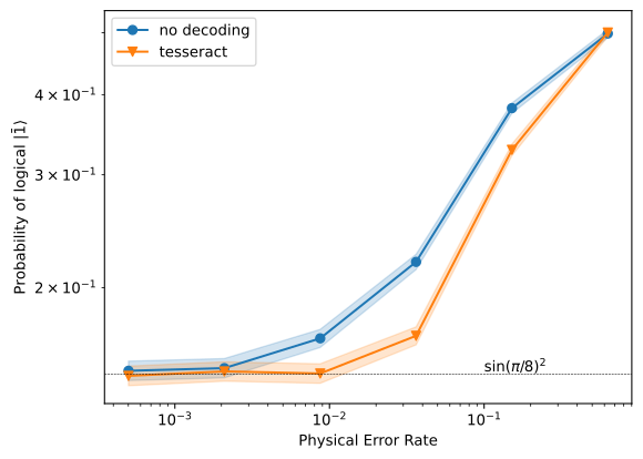
tsim is compatible with sinter, a tool for performing large Monte Carlo simulations. We can use sinter to sample and decode over a range of physical error rates.

tesseract_dec = TesseractSinterDecoder()
no_dec = NoDecoder()

tasks = [
    sinter.Task(
        circuit=make_circuit(noise).cast_to_stim(),
        json_metadata={"p": noise},
    )
    for noise in np.logspace(-3.3, -0.2, 6)
]

collected_stats = sinter.collect(
    num_workers=1,
    tasks=tasks,
    decoders=["tesseract", "no decoding"],
    max_shots=1024 * 64,
    max_errors=1024 * 64,
    custom_decoders={"tesseract": tesseract_dec, "no decoding": NoDecoder()},
    start_batch_size=1024 * 64,
    max_batch_size=1024 * 64,
)

sinter provides a number of convenient plotting tools. Here, we use them to plot the observable flip rate as a function of the physical error rate. We observe that the decoded probability approaches the expected value of $\sin(\pi/8)^2$ much faster.

fig, ax = plt.subplots(1, 1)
sinter.plot_error_rate(
    ax=ax,
    stats=collected_stats,
    x_func=lambda stats: stats.json_metadata["p"],
    group_func=lambda stats: stats.decoder,
)
ax.loglog()
ax.set_xlabel("Physical Error Rate")
ax.set_ylabel(f"Probability of logical $|\\bar{1}\\rangle$")
ax.axhline(np.sin(np.pi / 8) ** 2, color="k", linestyle="--", lw=0.4)
ax.text(0.1, np.sin(np.pi / 8) ** 2 * 1.01, "$\\sin(\\pi/8)^2$", fontsize=10)
ax.legend();